Now Reading: Arrays in Data Structures: Complete Guide with Real-Life Examples
- 01
Arrays in Data Structures: Complete Guide with Real-Life Examples
Arrays in Data Structures: Complete Guide with Real-Life Examples
Written by Hamza Sanaulla
Arrays in Data Structures: Complete Guide with Real-Life Examples. Imagine walking into a massive Amazon fulfillment center. Millions of packages are spinning down conveyor belts, getting sorted, and flying out the door. How does the system keep track of all these items without collapsing into pure chaos? It doesn’t just toss information into a digital pile. Instead, it relies on strict, predictable systems to keep data organized.
When you dive into software development, you quickly realize that your code faces the same challenge. If you throw data into random, scattered corners of your computer’s memory, your application will crawl to a painful halt. That is where data organization techniques come into play.
If you are beginning your coding interview preparation or simply want to master algorithm design, there is one foundational concept you cannot skip: the array data structure. It is the absolute bedrock of modern data handling methods. Let’s peel back the layers of this essential programming building block, explore how it interfaces with physical hardware, and look at how it solves real-world engineering problems.
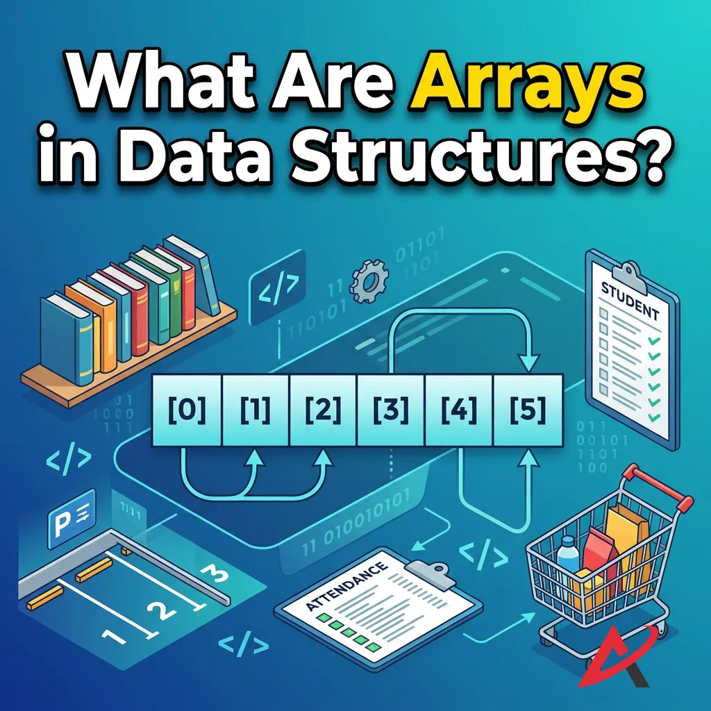
What Are Arrays in Data Structures?
When people first venture into a data structures course, they are often bombarded with overly complex, academic jargon. Let’s strip all of that away. What is an array in data structure terminology? Simply put, it is the digital equivalent of a cleanly divided pill organizer or a perfectly straight row of numbered storage lockers. Every single locker is identical in size; they are bolted tightly against each other in a single line, and they are designed to hold the same type of object.

Strategy for keeping related pieces of information grouped cleanly. Rather than creating ten separate variables to store ten different numbers, which would make your codebase an absolute nightmare to maintain, you bundle them into a single, cohesive unit. This structure isn’t just an arbitrary design choice; it is a fundamental pillar of computer science that influences how operating systems, engines, and modern applications manage data at scale.
Definition of an Array
To be technically precise, an introduction to arrays requires a strict definition: an array is a linear collection of elements of the same data type stored in perfectly contiguous memory locations.
Let’s break down those three non-negotiable rules:
- Collection of Elements: It bundles multiple individual items together under a single identifier name.
- Same Data Type: It enforces strict homogeneity. If you declare an array to hold integers, it can only hold integers. You cannot casually drop a text string or a decimal floating-point number into the middle of a compiled integer array.
- Contiguous Alignment: The items are physically placed back-to-back inside your computer’s Random Access Memory (RAM). There are zero gaps, zero fragments, and no empty spaces between the slots.
Why Arrays Are Important in DSA
Why does every comprehensive DSA learning guide place arrays on page one? Because you cannot build complex systems without understanding them first. More advanced data structures, such as hash tables, heaps, matrices, and string buffers, are frequently built using arrays under the hood.
Furthermore, if you are actively working on array problem solving for an upcoming technical screening, you will find that top-tier tech companies use array-based questions to test your core understanding of memory utilization and runtime performance. It is the gold standard for evaluating a candidate’s grasp of basic programming logic.
Basic Characteristics of Arrays
To fully understand what an array in data structures is, keep these four core traits in mind:
- Fixed Configuration: Once you define the size of a standard array, it is locked in. If you request a setup with five slots, it cannot magically expand to hold a sixth item without a complete overhaul.
- Sequential Data Storage: Data flows in a predictable, straight line. Element $B$ lives exactly one slot after Element $A$.
- Homogeneous Nature: Every single element demands the same number of bytes in memory.
- Direct Accessibility: You don’t have to scan the entire collection from left to right to find a specific entry. If you know the position number, you can jump straight to it instantly.
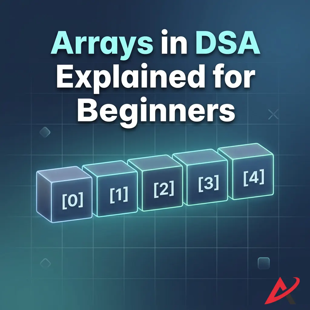
Arrays in DSA Explained for Beginners
For those exploring arrays in data structures for beginners, the trickiest part isn’t writing the code; it is visualizing what happens inside your machine’s hardware when that code executes. Let’s look at the mechanics of data storage in arrays to see how software interacts with physical memory chips.
How Arrays Store Data
When you tell your computer to create an array, it doesn’t just look for loose, scattered bits of free space across your RAM. It actively searches for a single, uninterrupted block of memory large enough to fit your entire request.
As a software engineer named Marcus Vance once noted:
Think of an array like a train. You can’t distribute the train cars across different tracks and expect it to function. They must be coupled together, sequentially, on a single line for the engine to move them efficiently.
This tightly coupled structure is precisely what makes arrays incredibly fast for certain tasks, yet rigid for others.
Understanding Indexing in Arrays
To retrieve data without errors, arrays use a system called array indexing. Each position inside the collection is assigned a specific numerical identifier. In almost all modern software development environments (such as C++, Java, Python, and JavaScript), arrays use zero-based indexing.
This means the very first item in your collection does not live at index 1; it lives at index 0. The second item sits at index1, the third at index2, and the final item rests comfortably at index n-1, where n represents the total capacity of your array. Skipping or forgetting this zero-based rule is the number one cause of the infamous “index out of bounds” error that plagues beginners during array exercises for beginners.
Memory Allocation in Arrays
To understand why zero-based indexing is used, we have to look at contiguous memory allocation. When an array is initialized, the computer records the exact memory address of the very first element. This starting point is known as the Base Address.
Because every slot in the array has the same data type, the computer knows precisely how many bytes each item consumes. Let’s say you create an integer array in C++ or Java. On most modern systems, a standard integer takes up exactly 4 bytes of memory.
If your array starts at the base address 2000, the memory management in arrays carves out the hardware blocks like this:
| Index | Element | Physical Memory Address Calculation | Actual Address |
| 0 | First | $\text{Base Address} + (0 \times 4 \text{ bytes})$ | 2000 |
| 1 | Second | $\text{Base Address} + (1 \times 4 \text{ bytes})$ | 2004 |
| 2 | Third | $\text{Base Address} + (2 \times 4 \text{ bytes})$ | 2008 |
| 3 | Fourth | $\text{Base Address} + (3 \times 4 \text{ bytes})$ | 2012 |
Notice the mathematical elegance here. The index number isn’t just an arbitrary label; it is a literal multiplier that tells the CPU exactly how many steps to skip from the base address. To find the item at index 3, the computer doesn’t inspect the index 0, 1, or 2. It performs a single multiplication: $2000 + (3 \times 4) = 2012$, and jumps directly to that address. This capability is called random access or index-based access, and it ensures efficient data retrieval regardless of how large the collection grows.
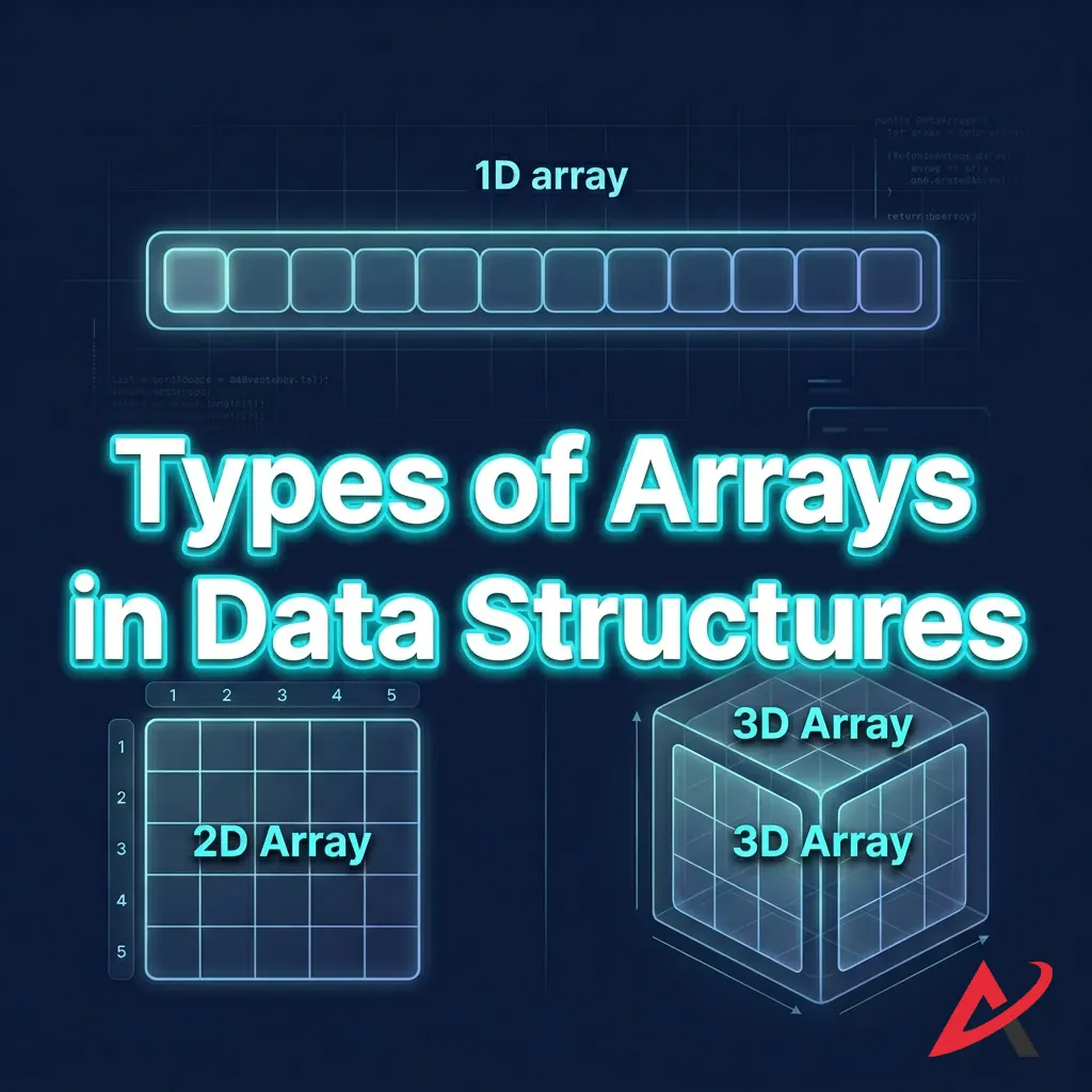
Types of Arrays in Data Structures
As software requirements grew more complex over the years, engineers realized that a single style of array couldn’t solve every problem. Today, we categorize these structures into a few distinct types of arrays in data structures based on their dimensions and how they manage memory limits.
One-Dimensional Arrays
The one-dimensional array (often called a 1D array or a linear vector) is the simplest variant available. It stores data in a single horizontal row. If you are writing an application to hold a list of weekly expenses or user IDs, a 1D array is your go-to option.
- Array Syntax & Declaration: In a language like C, you write
int expenses[7];. To see how fixed arrays operate natively at a low language level, you can review the ISO C Standard Array Specifications. - Array Initialization: You fill the slots instantly:
int expenses[7] = {50, 20, 45, 12, 90, 65, 30};.
Two-Dimensional Arrays
When your data demands a grid structure rather than a simple line, you scale up to a two-dimensional array (a 2D array). Think of a 2D array as a spreadsheet or a matrix complete with horizontal rows and vertical columns.
To locate a specific item inside a 2D array, you must provide two coordinates instead of one: array[row_index][column_index]. Behind the scenes, your computer’s physical memory is still strictly linear. The operating system flattens this grid into a single line using a method called Row-Major Order (storing row 0 entirely, followed by row 1, and so on) or Column-Major Order.
Multi-Dimensional Arrays
You can stack arrays even further to create multidimensional arrays. A three-dimensional array (3D array) can be visualized as a cube of data or a stack of multiple 2D spreadsheets layered on top of each other. While you can technically create 4D, 5D, or even higher-dimensional structures, they become increasingly difficult to visualize and can rapidly consume vast amounts of memory if not managed carefully.
A unique subset worth noting here is jagged arrays. In a standard 2D array, every single row must have the same number of columns. A jagged array, however, is an array of arrays where each sub-array can have a completely different length. Row 0 might contain 2 items, while Row 1 contains 15 items.
Dynamic Arrays
Standard arrays are inherently static; their size is set at launch and cannot change. This poses a major challenge if you don’t know how much data your users will input. To solve this, languages utilize the dynamic array.
When you use a dynamic array, such as a list in Python or an ArrayList in Java, the language engine manages a hidden static array under the hood. For a breakdown of how this memory reallocation functions under the hood in Java environments, check out the official Oracle Java ArrayList Documentation.
The moment your data outgrows this hidden layout, the system executes a clever trick:
- It allocates a brand-new, independent block of memory that is typically double the size of the original.
- It copies all existing array elements over to the new block.
- It safely deletes the old, cramped array block to free up system memory.
This automatic adjustment provides the flexibility of fluid resizing while retaining the rapid lookup speeds of traditional array structures.
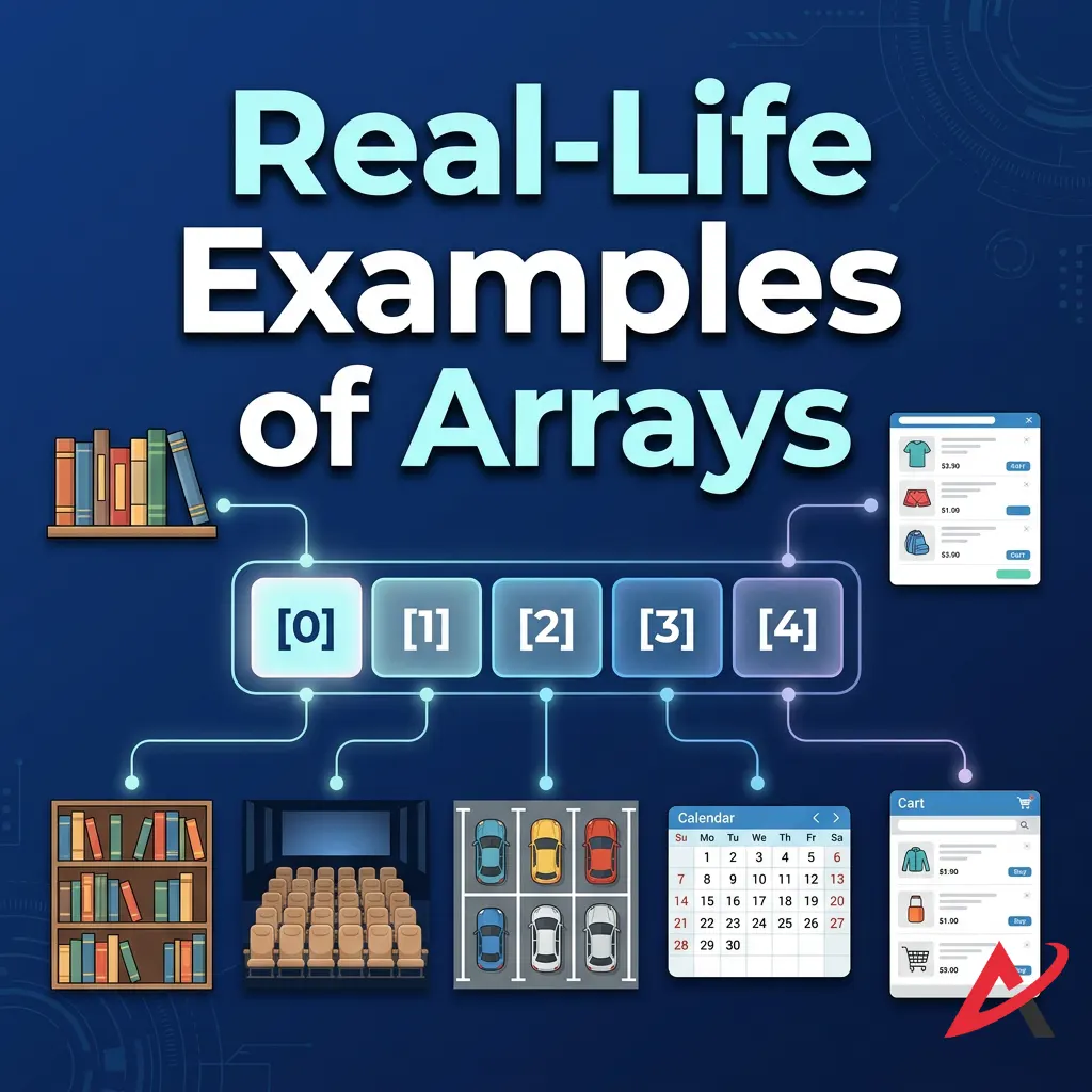
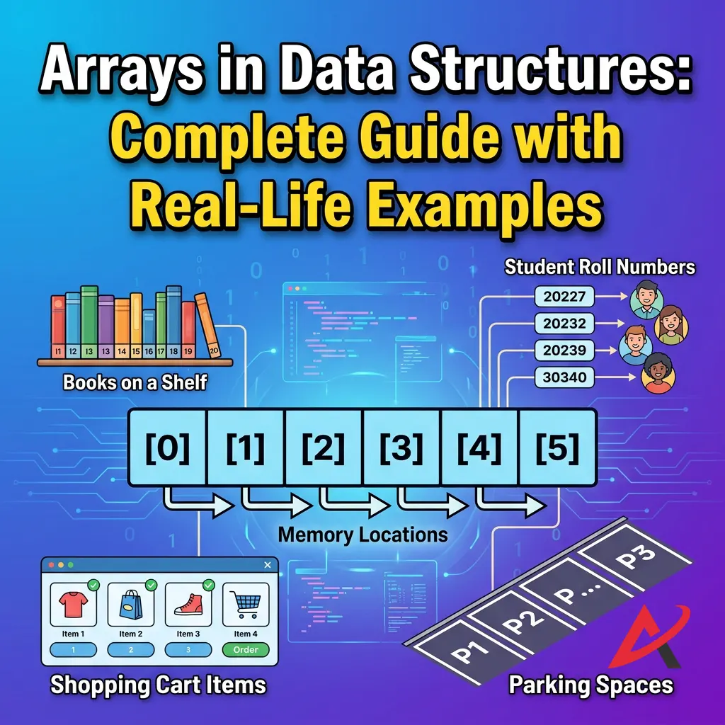
Real-Life Examples of Arrays
To see why arrays are so fundamental to software development, let’s look at a few real-life examples of arrays in DSA that you likely interact with every single day.
Student Records Management
In a school grading database, a school counselor might use a 1D array to manage a student’s semester test scores. Because a semester has a fixed number of scheduled exams, using a static array ensures that the scores are stored cleanly in chronological order without wasting unnecessary system resources.
Storing Daily Temperatures
Meteorology programs use arrays to log continuous atmospheric data. For example, a weather station tracking the highest temperature for each hour of a 24-hour cycle will store those 24 decimal values in a linear array. The index number maps directly to the hour of the day (e.g., temp[0] is midnight, temp[13] is 1:00 PM).
Product Lists in E-Commerce
When you open an app like Amazon or eBay, the horizontal product carousels displaying “Recommended Items for You” are driven by arrays. The system pulls a set number of product objects from a database and lines them up sequentially inside an array to render them across your screen.
Image Pixel Representation
Every digital image on your monitor or phone screen is powered by a 2D or 3D array. A basic grayscale image is a 2D array where each element represents a specific pixel’s brightness value from 0 (black) to 255 (white). For full-color digital photos, applications use a 3D array where the third dimension holds three separate layers for the Red, Green, and Blue (RGB) color channels.
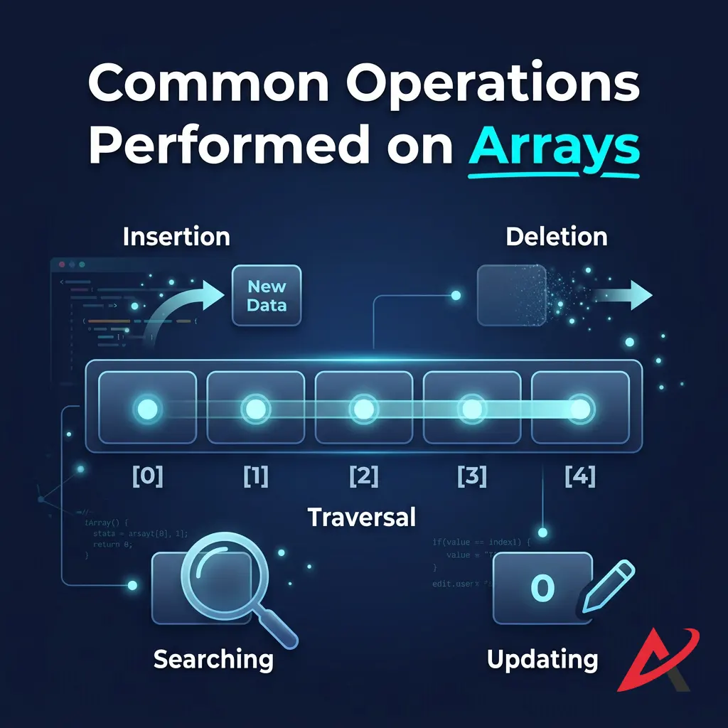
Common Operations Performed on Arrays
To write clean software and excel in competitive programming arrays, you need to understand the mechanics of fundamental array operations. Let’s examine how these operations manipulate data behind the scenes.
Array Traversal
Traversing arrays is the foundational process of systematically moving through the collection from index 0 all the way to the end. You use traversal whenever you need to print every item to a console, search for a specific value, or modify every entry in the list.

Insertion in Arrays
Adding a new element to an array depends heavily on where you want to put it.
- Insertion at the End: If you are using a dynamic array with open slots, adding an item to the very end is simple. You drop the value into the next available index.
- Insertion at the Start or Middle: If you want to insert a value at index
0, you cannot simply overwrite the existing data. You have to manually shift every single element one slot to the right to make room for the new arrival. This shifting requirement makes mid-array modifications computationally expensive.
[Image demonstrating array insertion where elements shift right to accommodate a new item at index 1]
Deletion from Arrays
Much like insertion, deletion from arrays requires careful cleanup to maintain a solid, unbroken block of data. If you delete an item from the middle of an array, you cannot leave a blank gap in a contiguous structure. You must take every element to the right of the deleted item and shift it one slot to the left to close the vacancy.
Searching Elements
If you need to find a specific value inside an unorganized array, you must perform a Linear Search. This involves checking every single item one by one from the beginning until you find a match. However, if your array has been organized using array sorting algorithms, you can unlock a much faster method called Binary Search. This approach cuts your search zone completely in half with each step, allowing you to find items in a fraction of the time.
Updating Array Values
Updating an item is the fastest operation you can perform on an array. Because you don’t need to change the size or shift any surrounding data, you can overwrite a value instantly if you know its index position: arr[2] = 99;.
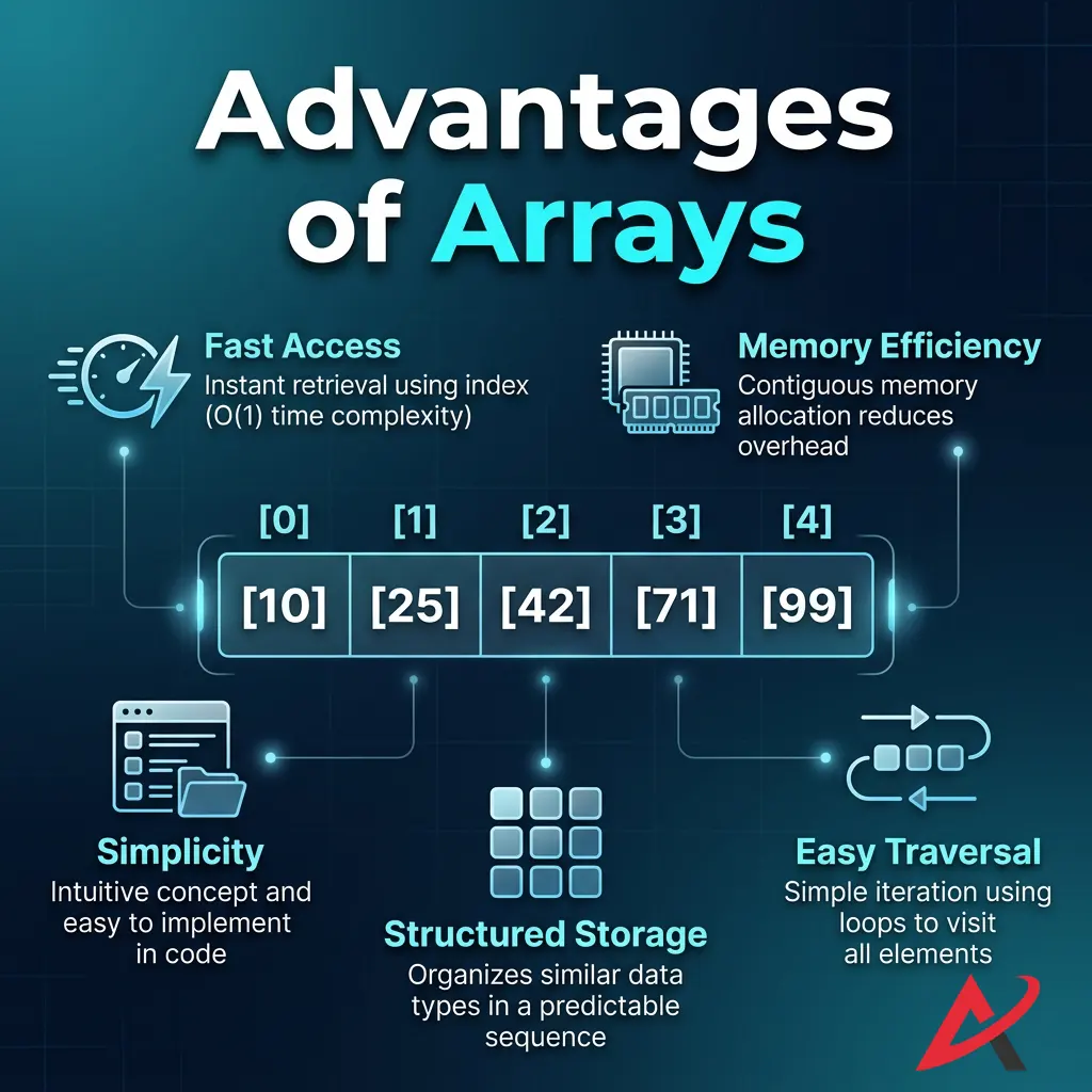
Advantages of Arrays
Every data layout comes with architectural trade-offs. Let’s look at the key advantages that make arrays an essential choice for software engineers.
- Fast Data Access Thanks to index-based random access math, looking up any element takes the same amount of time, whether your array contains 5 items or 5 million items.
- Easy Implementation: Arrays feature incredibly clean syntax across almost every programming language, requiring minimal setup or boilerplate code compared to custom structures.
- Efficient Memory Usage Because arrays store data back-to-back in a single block, they use memory very efficiently. They don’t waste extra bytes storing structural links or pointers like those found in alternative designs.
- CPU Cache Friendliness Modern computer processors love contiguous memory blocks. When a CPU reads an array element, it automatically pre-fetches the neighboring elements into its ultra-fast cache memory, resulting in blazing-fast execution speeds.
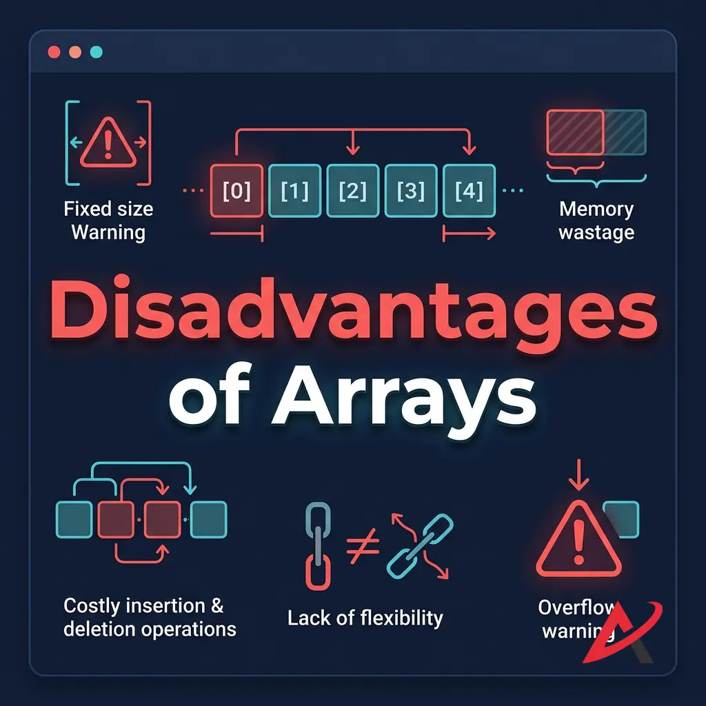
Disadvantages of Arrays
To avoid introducing bugs into your applications, it’s equally important to understand where arrays struggle.
- Fixed Size Limitation: With standard static arrays, you must declare your maximum size up front. If you underestimate your data needs, your program can crash; if you over-allocate, you end up wasting valuable system resources.
- Costly Insertions and Deletions. As we explored in our operations breakdown, inserting or deleting items from the middle of an array requires shifting large blocks of data, which can slow down performance on larger datasets.
- Memory Wastage Issues: If you allocate an array to hold 10,000 user profiles but only 100 people register, the remaining 9,900 slots sit empty while permanently holding onto that allocated memory block.
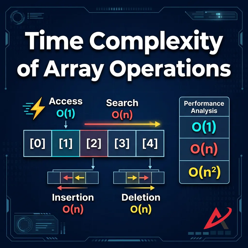
Time Complexity of Array Operations
When evaluating algorithms for a data structures training program, we measure efficiency using Big-O notation. Here is the standard runtime performance profile for core array operations:
| Operation | Best Case | Worst Case / Big-O | Structural Explanation |
| Access (by Index) | $O(1)$ | $O(1)$ | Direct mathematical jump via base address calculations. |
| Search (Linear) | $O(1)$ | $O(n)$ | Happens when the target item sits at the very end of the list. |
| Search (Binary) | $O(1)$ | $O(\log n)$ | Requires the array to be sorted beforehand. |
| Insertion | $O(1)$ | $O(n)$ | The worst case occurs at index 0, requiring every element to shift left. |
| Deletion | $O(1)$ | $O(n)$ | Worst case occurs at index 0, requiring every element to shift left. |
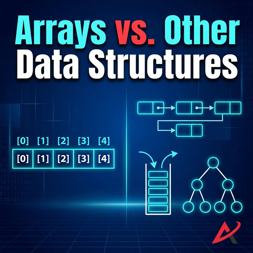
Arrays vs. Other Data Structures
Choosing the right tool for the job is a core skill in software development. Let’s see how arrays compare to other popular options you’ll find in an online DSA tutorial.
Arrays vs. Linked Lists
A linked list does away with contiguous memory entirely. Instead, it scatters data nodes across random locations in your RAM, connecting them like a chain using memory pointers.
- The Trade-off: Linked lists allow for instant insertions and deletions without any data shifting. However, they lose the ability to perform random lookups; to read the 50th item, you must walk through the first 49 nodes one by one.
Arrays vs. Stacks
A stack is a specialized container that follows a strict Last-In, First-Out (LIFO) order, similar to a stack of dinner plates in a cafeteria. You can only interact with the very top item. Arrays, by contrast, give you total freedom to read or write to any index position at any time.
Arrays vs. Queues
A queue operates on a First-In, First-Out (FIFO) principle, much like a real-world waiting line at a grocery store counter. While you can implement a queue using an array under the hood, the queue structure limits direct access to ensure elements are processed in the exact order they arrived.
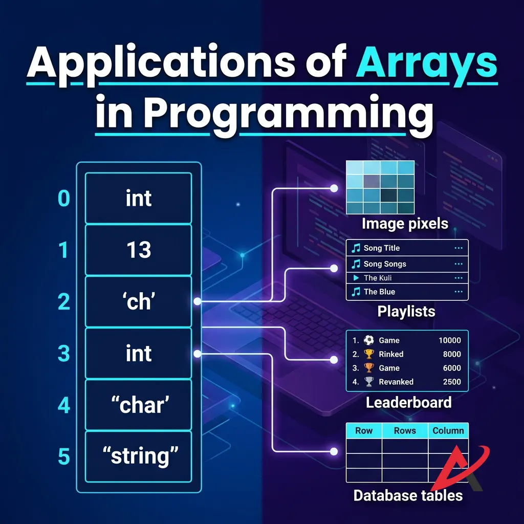
Applications of Arrays in Programming
Where do arrays do the heavy lifting in real-world commercial software? They power several foundational systems:
- Database Management Systems (DBMS): Databases frequently use array structures to build internal index directories, allowing them to locate specific data records on disk with minimal delay.
- Game Development: Game engines rely heavily on arrays to manage game world state—from tracking leaderboard scores and current player inventories to running loops that render graphics to your screen.
- Machine Learning and Data Analysis: Modern AI applications are built on linear algebra matrices. Under the hood, these data structures are represented as massive multidimensional arrays processing millions of mathematical operations simultaneously. To understand how arrays map to data analysis math, read the comprehensive NumPy Array Foundation Guide.
- Operating Systems: Your computer’s operating system uses internal arrays to manage active tasks, keep track of open files, and coordinate hardware devices and drivers.

Choosing the Right Learning Path: How to Master Array DSA
If you are looking to accelerate your engineering career, simply reading about arrays isn’t enough—you need a structured practice plan. Choosing how you study depends entirely on your personal learning style:
1. Hands-on Coding Platforms
If you learn best by doing, jump into DSA practice problems on platforms like LeetCode or HackerRank. Start with foundational array coding challenges like reversing an array or finding duplicates, then move on to advanced patterns like two-pointer sweeps and sliding windows.
2. Comprehensive Literature
If you want a deep dive into the underlying architecture, picking up the best data structures book for your language of choice will help you master the core mathematical concepts. A universally recommended text is Introduction to Algorithms by Thomas H. Cormen, Charles E. Leiserson, Ronald L. Rivest, and Clifford Stein.
3. Guided Video Modules
For visual learners, enrolling in a dedicated DSA certification course or following an interactive online DSA tutorial provides structured, step-by-step guidance to master these concepts efficiently.

Quick Summary / Key Takeaways
Before we conclude, let’s recap the vital core concepts to remember:
- Arrays provide incredibly fast index-based access ($O(1)$ time complexity) because they use a contiguous memory allocation model.
- The trade-off for that speed is rigidity: arrays have a fixed size and require slow element shifting ($O(n)$ time complexity) for insertions or deletions in the middle.
- Choose standard static arrays when your dataset size is predictable, and opt for dynamic arrays when your application needs to handle fluid, unpredictable amounts of data.
Conclusion
Key Takeaways About Arrays in DSA
At the end of the day, the array data structure remains an indispensable tool in modern computer programming. Its combination of predictable hardware placement, high-speed index access, and memory efficiency makes it the foundational building block upon which more complex data structures are created.
When to Use Arrays in Programming
When you sit down to design your next application, remember this simple rule of thumb: reach for an array whenever your data items are closely related, share the same data type, and require fast lookup speeds. As long as you don’t need to perform frequent insertions or deletions throughout the middle of your list, an array will deliver excellent performance.
Keep practicing your coding challenges, pay close attention to your index boundaries, and use arrays’ predictable speed to build faster, cleaner applications!
Related Blogs
What is DSA? Why Every Programmer Must Learn Data Structures and Algorithms
Time Complexity and Big O Notation Explained Like You’re 10 Years Old
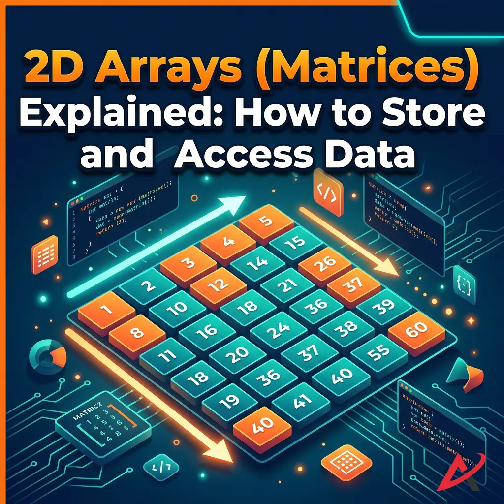
2D Arrays (Matrices) Explained: How to Store and Access Data